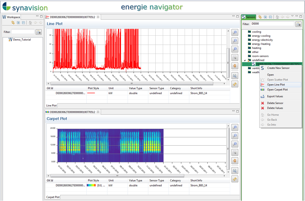
For the visualization of sensors and virtual sensors, four different plot patterns are available:
In the visualization of the selected function, rule, state, etc. the following buttons with different options appear next to the plot:
![]()
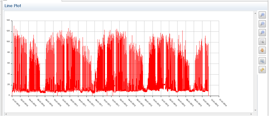
![]() Line Plots show the chronological trend of data. They can be used to display performance data, consumption, load profiles and results of functions and rules. The example on the right hand side shows the line plot of a power consumption over several years.
Line Plots show the chronological trend of data. They can be used to display performance data, consumption, load profiles and results of functions and rules. The example on the right hand side shows the line plot of a power consumption over several years.
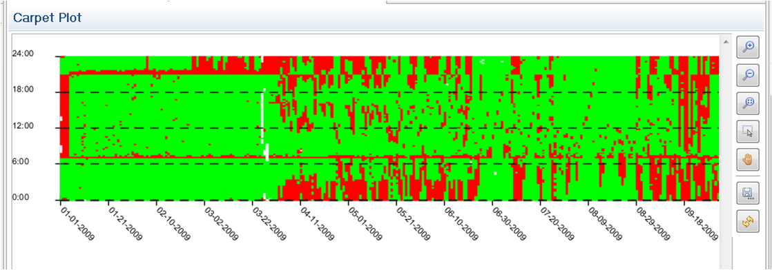
![]() Carpet Plots show temporal relation of visualised data. Each data point will be inscribed in a coordinate system. The abscissa shows a daily resolution whereas the ordinate has the resolution chosen in the workspace (one value per minute, quarter of an hour, hour or day). Carpet Plots are suitable especially for the visualization of operation performances and states, as well as to display the results of rules. The given example shows the evaluation of a state space according to TRUE (green) and FALSE (red).
Carpet Plots show temporal relation of visualised data. Each data point will be inscribed in a coordinate system. The abscissa shows a daily resolution whereas the ordinate has the resolution chosen in the workspace (one value per minute, quarter of an hour, hour or day). Carpet Plots are suitable especially for the visualization of operation performances and states, as well as to display the results of rules. The given example shows the evaluation of a state space according to TRUE (green) and FALSE (red).
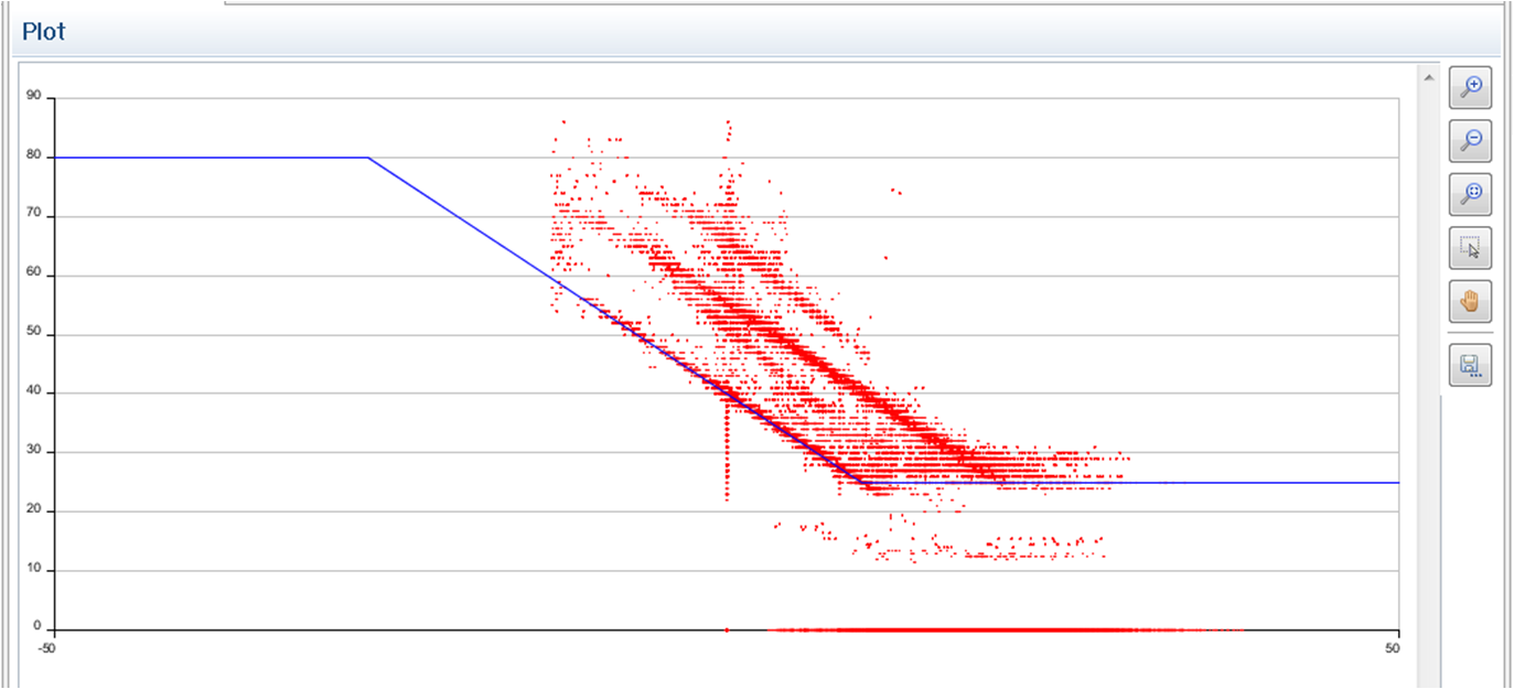
![]() Scatter Plots visualize the data by point clouds (x,y-graphic). By these kind of plots, relations between two data sets can be examined. One example could be to display the characteristic of a supply temperature according to the ambient temperature (blue) in combination with operational data (supply temperature, ambient temperature). It would also be possible to derive the course of a characteristic from a scatter plot showing the supply temperature in relation to the ambient temperature.
Scatter Plots visualize the data by point clouds (x,y-graphic). By these kind of plots, relations between two data sets can be examined. One example could be to display the characteristic of a supply temperature according to the ambient temperature (blue) in combination with operational data (supply temperature, ambient temperature). It would also be possible to derive the course of a characteristic from a scatter plot showing the supply temperature in relation to the ambient temperature.
![]() Cummulative curves are duration curves, that arrange the values of a data point/sensor over the whole time period, according to its amount of undercutting. Therefore the ordinate enables for every value, to identify the number of points in time, where this corresponding value has been undercut.
Cummulative curves are duration curves, that arrange the values of a data point/sensor over the whole time period, according to its amount of undercutting. Therefore the ordinate enables for every value, to identify the number of points in time, where this corresponding value has been undercut.

Data can be opened in the editor windowin form of line plots, cumulative curves or carpet plots, by right-clicking on the corresponding sensor in the section „Data Points“, or by right-clicking on the corresponding element (e.g. rule, function, metric) in the section „Specification“.
Additionally, the plot pilot can be used to create line-, bar-, scatter- and carpet plots, as well as performance charts. Multiple sensors can be added to the figure and the graphic can be edited at will. An URL will be assigned to every graphic in the plot pilot, which enables the integration of these graphics in external homepages and Word documents.